Particle Collisions Visualization (PV 5.4.1)
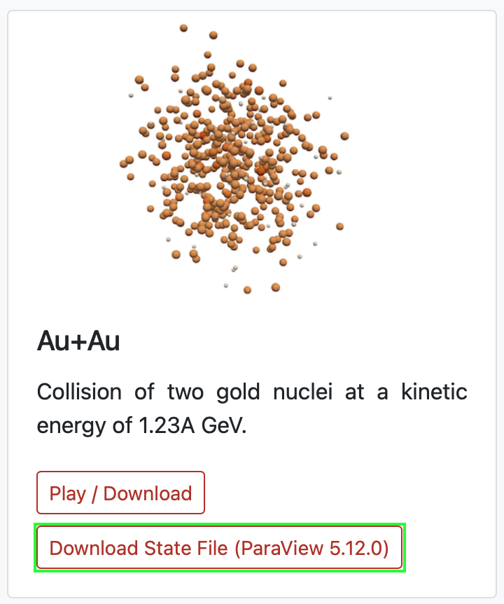
This section covers animating particles in an Au+Au collision. For this purpose, the needed SMASH output files can be downloaded here. Alternatively, you can run SMASH yourself using the config file AuAu_position_config.yaml. For an overview regarding SMASH output configuration options please refer to the official SMASH User Guide.
1. Open the File
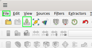
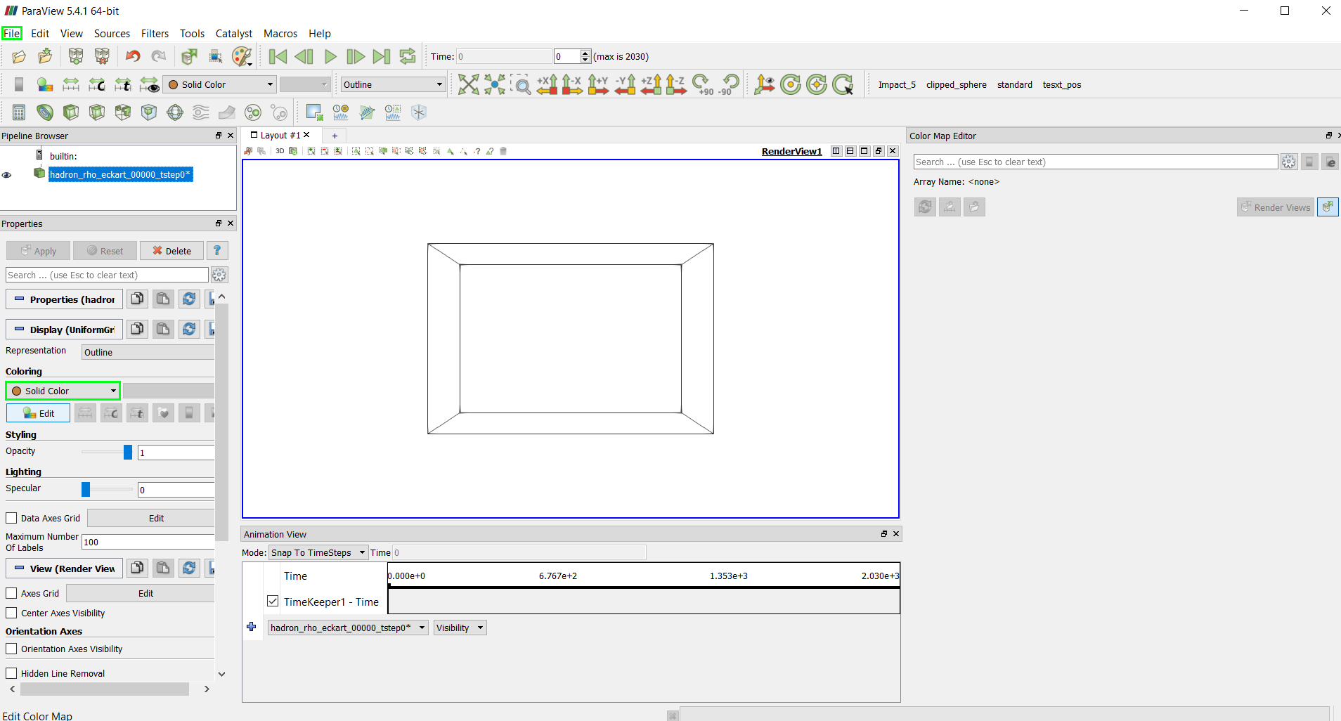
Open ParaView. Open the data file by clicking the File option in the top left corner of the Menu Bar, go to Open and choose the file called pos_ev00000_tstep..vtk in the position_data folder you have downloaded previously. The data set should be of the Type Group.
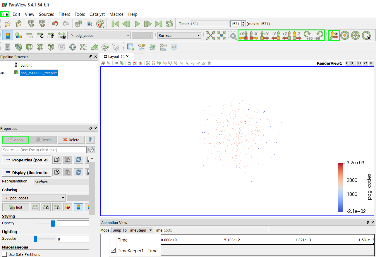
Click Apply ![]() in the Properties Panel. Data points and a color legend appear.
in the Properties Panel. Data points and a color legend appear.
On the left side in the Properties panel, set Background to Solid Color and choose a background color you like. Use the Camera Controls  and
and  to get a side view of the collision. Note that with the Show Orientation Axes
  button you can hide the little coordinate system.
2. Set Mass Dependent Scaling
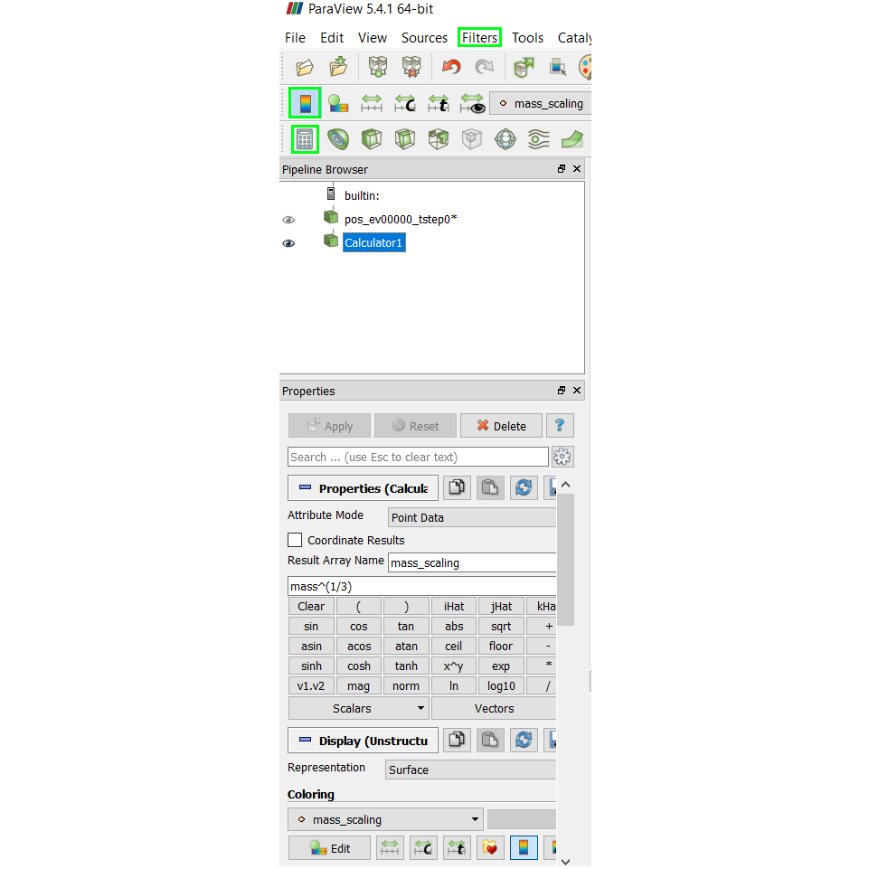
Later, we want the sizes of the particles to correspond to their weight according to V ∼ m⅓. The mass itself is a variable already contained in the SMASH data, so we only need to rescale it. To do so, we choose the Calculator ![]() option in the filter bar above the Pipeline Browser in the left corner (or go to Filters → Alphabetical→ Calculator). Type mass_scaling into the Result Array Name line and enter mass^(1/3) into the calculation field.
option in the filter bar above the Pipeline Browser in the left corner (or go to Filters → Alphabetical→ Calculator). Type mass_scaling into the Result Array Name line and enter mass^(1/3) into the calculation field.
Then press ![]() .
.
We have now created a new variable that is called mass_scaling and whose magnitude is defined by the third root of the respective particle's mass. Press Toggle Color Legend Visibility ![]() to get rid of the color legend.
to get rid of the color legend.
3. Add Glyphs
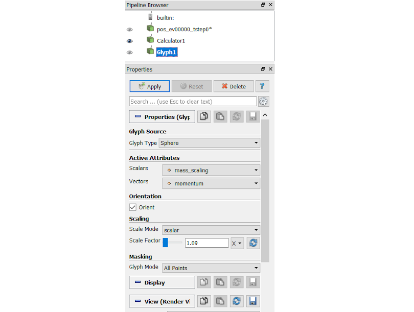
Choose the Glyph ![]() option in the filter bar or go to Filters → Alphabetical → Glyph. In the properties window, change Glyph Type to Sphere. In the Active Attributes section, make sure Scalars is set to mass_scaling. In the Scaling section, set Scale Mode to scalar and choose a Scale Factor to your liking, for example 1.09. This will define the size of the visualized nucleons. We want to show all nucleons, so we have to change Glyph Mode in the Masking section to All Points.
option in the filter bar or go to Filters → Alphabetical → Glyph. In the properties window, change Glyph Type to Sphere. In the Active Attributes section, make sure Scalars is set to mass_scaling. In the Scaling section, set Scale Mode to scalar and choose a Scale Factor to your liking, for example 1.09. This will define the size of the visualized nucleons. We want to show all nucleons, so we have to change Glyph Mode in the Masking section to All Points.
Press ![]() .
.
Everything else is now completely up to your liking!
4. Legend and Colors
Next, we will try to make the movie look actually visually appealing. This means, for example, adding units and labels to the legend. Also, you may note that the coloring scheme of our particles is currently diverging which is not necessarily appropriate for a linearly scaling unit such as the mass.
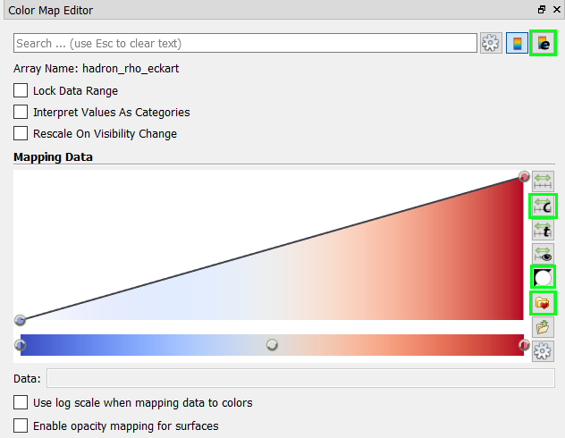
So let us start by improving our legend. First, look at the Pipeline Browser and make sure that Glyph1 is selected (recognizable by the blue border around it – this is also called the active view). Now, if not already visible, press the Color Map Editor ![]() button (or go to View and check Color Map Editor). Within the now opened window click the Edit Color Legend Properties
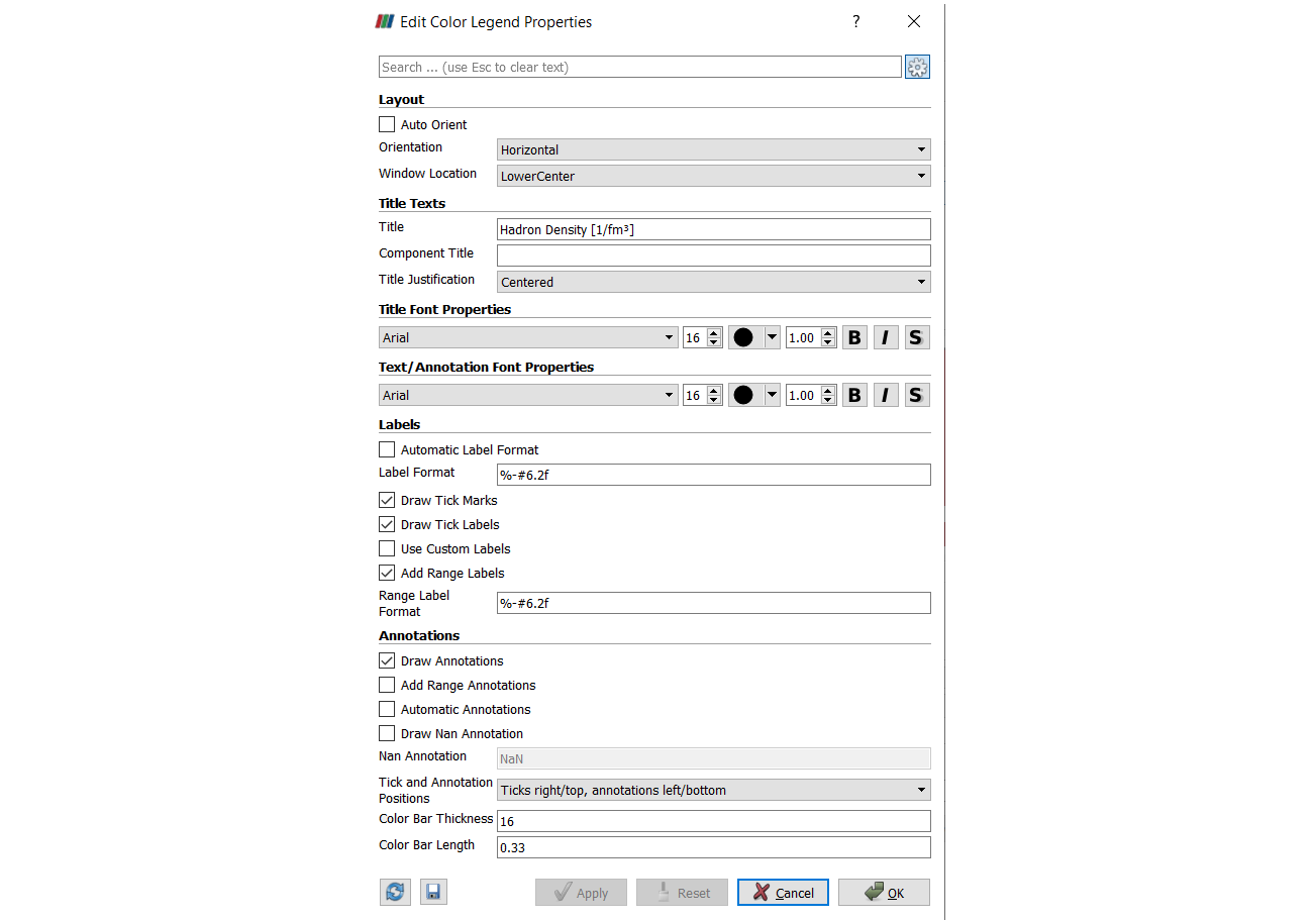
button (or go to View and check Color Map Editor). Within the now opened window click the Edit Color Legend Properties ![]() button. Capitalize the title and add the unit [GeV] to it, and set all font properties to the color black (or white depending on your background color). You may want to play around with the other settings in order to get know them and find out what you like.
button. Capitalize the title and add the unit [GeV] to it, and set all font properties to the color black (or white depending on your background color). You may want to play around with the other settings in order to get know them and find out what you like.
Press ![]() to see the changes you have made. If you are content with your choices, press
to see the changes you have made. If you are content with your choices, press ![]() .
.
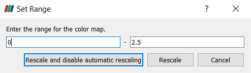
Pressing the Rescale to custom range ![]() button, you can set the range of the color bar, for example from 0 to 2.5.
button, you can set the range of the color bar, for example from 0 to 2.5.
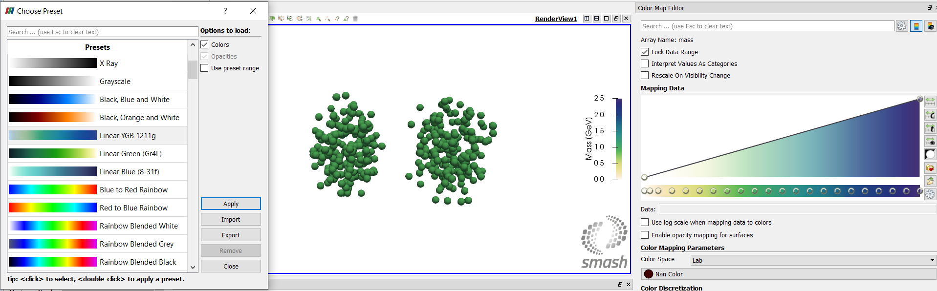
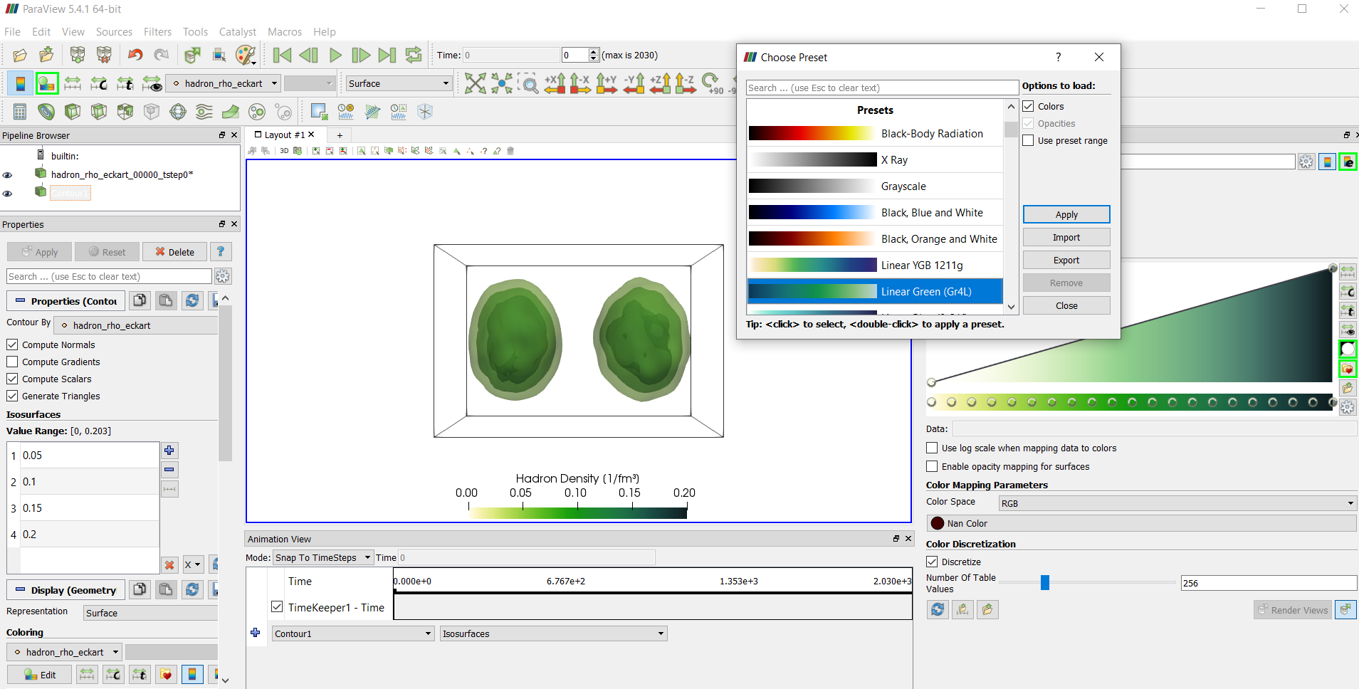
To change the diverging coloring scheme of our particles, click on the Choose preset ![]() button (you might have to enlarge the width of the Color Map Editor sidebar for this button to be visible). Choose any preset you like and press
button (you might have to enlarge the width of the Color Map Editor sidebar for this button to be visible). Choose any preset you like and press ![]() to see the changes. When you are finished, press
to see the changes. When you are finished, press ![]() .
.
5. Text and Clock
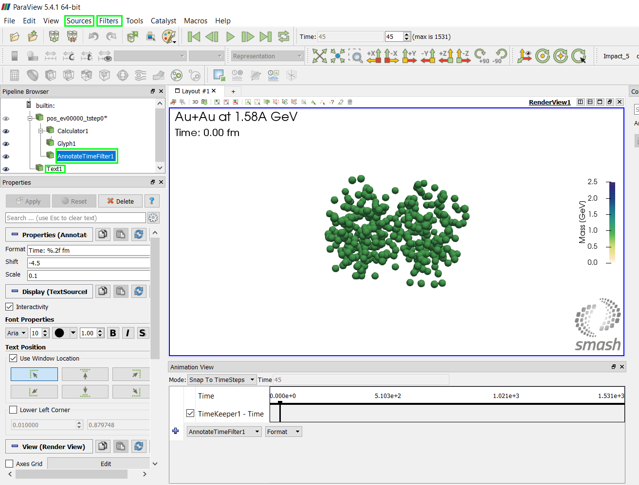
Let's add titles and a clock! To add writing, go to Sources → Text. Type whatever you like into the text field and press ![]() . Now you can modify the color, size and positioning of your text in the Properties panel.
. Now you can modify the color, size and positioning of your text in the Properties panel.
To add a clock go to Filters → Temporal → Annotate Time Filter. In the Properties panel set Format to Time: %.1f fm (in newer ParaView versions the formatting has changed to: Time: {time:.1f} fm). In our provided data set, we have chosen an output interval of 0.1, so we have to change Scale to 0.1. Since in SMASH the time starts counting when the first particle collision happens, we have to set Shift to -4.5. Press ![]() . Change the position, size and color of the clock to your liking.
. Change the position, size and color of the clock to your liking.
6. Save your Animation
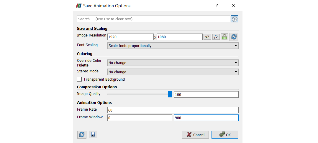
Lastly, you will probably want to save your animation. Go to File → Save Animation. Set the Image Resolution to 1920×1080 – this is the standard movie format, you can choose any format you like. The overall look and positioning of the text may look different when changing this.
Now look at the Animation Options down below. Increase the Frame Rate to 60, or at least 30. This will determine how many frames per second will be played in your animation and, ultimately, sets the speed and duraion of your movie. A typical frame rate in movies is 24 frames per second, but since our original timesteps are so small, a higher frame rate is needed. Once your are finished, you may still change the frame rate in post-production using any movie editor program available to you.
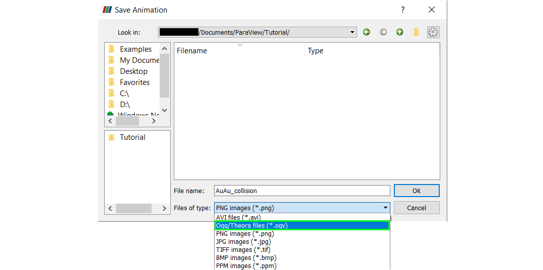
Set Frame Window from 0 to 600. Press ![]() . Give your animation a name. Change the format to Ogg/Theora files(*.ogv). Alternatively, you can also save all individual frames as image files and make them into movies using another movie making software. The specified frame rate has no consequence in that case, of course.
. Give your animation a name. Change the format to Ogg/Theora files(*.ogv). Alternatively, you can also save all individual frames as image files and make them into movies using another movie making software. The specified frame rate has no consequence in that case, of course.
Congratulations, you have now made your first movie with ParaView!
 .
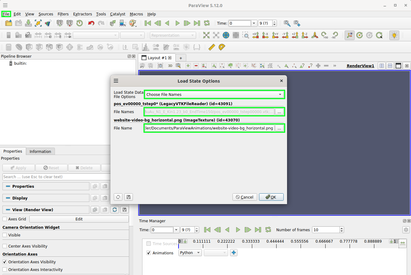
ParaView must be able to find all of these files or will prompt you with error messages after clicking
.
ParaView must be able to find all of these files or will prompt you with error messages after clicking